Modeling of Geometric Nonlinearity in Tank Shell and Base Plate

Next: Proposed Finite Element Modeling Up: The Finite Element Technique Previous: Variational Principles of the

Modeling of Geometric Nonlinearity in Tank Shell and Base Plate

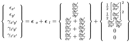
The majority of failures in unanchored liquid storage tanks during past earthquakes occurred because of shell buckling near the tank base. This failure mode is caused by the seismic overturning moment resulting from the hydrodynamic pressures exerted by the liquid in addition to axial stress concentration resulting from base plate uplift. Hence, geometric nonlinear terms were incorporated in formulations of the degenerated shell element used to model the tank as follows

$\displaystyle {\mbox{\boldmath$\epsilon$ }}$	=	$\displaystyle \left\{\begin{array}{c} \epsilon_{x'}\\ \epsilon_{y'}\\ \gamma_... ... w'}{\partial x'}\frac{\partial w'}{\partial y'}\\ 0\\ 0 \end{array} \right\}$	(7)
	=	$\displaystyle \sum_{i=1}^n \left( {\bf B}_{o} + {\bf B}_{l} \right)_i \left\{\b... ...{c} \overline{{\bf u }}_i \\ {\mbox{\boldmath$\theta$ }}_i \end{array}\right\}$	(8)

where ${\bf B}_o$ is the linear strain-displacement matrix and ${\bf B}_l$ is the nonlinear strain-displacement matrix. In order to find ${\bf B}_l$ , the nonlinear strain component is rewritten as

$\begin{displaymath}\mbox{{\boldmath$\epsilon$ }}_l = \frac{1}{2} \left[\begin{a... ...\} =\frac{1}{2} \left[ D \right] \left\{ \epsilon_{c} \right\} \end{displaymath}$

(9)

where $\epsilon_{c}$ is the strain vector that couples the membrane strain to the out of plane displacements. These coupling strains are related to the nodal degrees of freedom by

$\begin{displaymath}\mbox{{\boldmath$\epsilon$ }}_{c} = \sum_{i=1}^n \left[\begi... ... u}_i \\ \mbox{{\boldmath$\theta$ }}_i \end{array} \right\} \end{displaymath}$

(10)

The matrix ${\bf B}_l$ is then given by

$\displaystyle \left[B_l\right]_i$	=	$\displaystyle \left[D\right]_i \left[\begin{array}{cc} {\bf G}^u&{\bf G}^\theta \end{array} \right]_i$
	=	$\displaystyle {\bf D}_i \; {\bf G}_i$	(11)
$\displaystyle {\bf G}^u$	=	$\displaystyle \left[ \begin{array}{ccc} 0 & 0 & \frac{\partial N_i}{\partial x'... ... 0 & 0 & \frac{\partial N_i}{\partial y'} \end{array}\right] \left [ q \right]$	(12)
$\displaystyle {\bf G}^\theta$	=	$\displaystyle \frac{t_i}{2} \left[ \begin{array}{ccc} 0& 0 & \frac{ \partial \l... ..._i \right) }{\partial y'} \end{array}\right] \left [ q \right]\left[ R_i\right]$	(13)

In large deformation analysis, the strain vector is incrementally updated after each time step by

$\begin{displaymath}\delta \mbox{{\boldmath$\epsilon$ }} = \sum_{i=1}^{n} \left... ...\ \delta \mbox{{\boldmath$\theta$ }}_i \end{array} \right\} \end{displaymath}$

(14)

The stiffness matrix is then given by

$\begin{displaymath}\left[ K \right] =\int_{\Omega} \left [ \left[ B_o+B_l \right... ...a_{y'} \end{array} \right] \left[ G \right] \right] d\Omega \end{displaymath}$

(15)

Next: Proposed Finite Element Modeling Up: The Finite Element Technique Previous: Variational Principles of the

A. Zeiny
2000-05-12